10. 案例: 大豆异黄酮 MBMA#
基于模型的荟萃分析(model based meta-analysis,MBMA)是一种将定量药理学建模与荟萃分析(meta-analysis)相结合的分析方法。相较于群体 PK-PD 建模的方法而言,MBMA 可以整合多个来源(临床前和临床研究、个体数据和文献数据等)和维度(人口学特征、试验设计方案、给药方案等)的临床数据以解决单个临床研究难以回答的问题。MBMA 通过构建定量药理学模型可合并分析不同剂量、不同疗程和不同人群的数据并探索其中导致异质性的潜在因素,从而对药物的剂量-效应关系、时间-效应关系和影响因素进行定量化,并可基于模型预测以往研究中未涉及的剂量、时间或协变量水平下的药效特征,为药物研发各个关键环节的决策制定提供重要依据。MBMA 目前已经是模型引导的药物开发策略中的重要方法之一。
在本节中,我们将以大豆异黄酮治疗更年期潮热的模拟临床试验数据为例,操练 MBMA 的基本建模方法与熟悉整体分析流程。
参考文献
了解更多有关 MBMA 的知识:
李禄金, 丁俊杰, 刘东阳, 王曦培, 邓晨辉, & 季双敏等. (2020). 基于模型的荟萃分析一般考虑. 中国临床药理学与治疗学(025-011).
大豆异黄酮治疗更年期潮热 MBMA 文献:
Li, L., Lv, Y., Xu, L., & Zheng, Q. (2015). Quantitative efficacy of soy isoflavones on menopausal hot flashes. British journal of clinical pharmacology, 79(4), 593–604.
10.1. 数据探索#
我们可从
mas.datasets内导入大豆异黄酮 MBMA 示例数据soy_isoflavone:
from mas.datasets import soy_isoflavone
from mas.model import *

import polars as pl
soy_isoflavone.head(10)
| ID | TIME | DV | SAMPLE | AGE | BASELINE | CENTRE | YEAR |
|---|---|---|---|---|---|---|---|
| i64 | i64 | f64 | i64 | i64 | f64 | i64 | i64 |
| 1 | 0 | 0.0 | 159 | 36 | 3.8 | 1 | 1 |
| 1 | 12 | -20.0 | 159 | 36 | 3.8 | 1 | 1 |
| 2 | 0 | 0.0 | 135 | 41 | 3.6 | 0 | 1 |
| 2 | 8 | -51.6 | 135 | 41 | 3.6 | 0 | 1 |
| 3 | 0 | 0.0 | 105 | 42 | 6.3 | 0 | 1 |
| 3 | 1 | -49.0 | 105 | 42 | 6.3 | 0 | 1 |
| 3 | 2 | -68.0 | 105 | 42 | 6.3 | 0 | 1 |
| 3 | 3 | -77.0 | 105 | 42 | 6.3 | 0 | 1 |
| 3 | 4 | -82.3 | 105 | 42 | 6.3 | 0 | 1 |
| 3 | 5 | -86.0 | 105 | 42 | 6.3 | 0 | 1 |
数据内的各列分别代表:
ID:试验编号
TIME:观测时间(周)
DV:观测值,自基线的潮热发作频率下降率(%)
SAMPLE:试验的样本量
AGE:受试者平均年龄
BASELINE:基线时患者的平均潮热发作频率(次/天)
CENTRE:是否为多中心研究,0 代表单中心研究,1 代表多中心研究
YEAR:是否来源于近十年发表的文献,0 为否,1 为是
使用 plot_profile() 来观测数据趋势:
p_profile = plot_profile(soy_isoflavone)
p_profile
从上图可以发现,观测值数据有随时间变化而先下降后平稳的趋势(例如 ID=3 的数据),提示我们可以使用 Emax 模型作为基础模型进行建模。
备注
Emax 模型的公式为:
其中 Emax 为最大效应值,ET50 为达到 50% 最大效应所需的时间,ET50 越小则说明起效越快(图 10.1)。
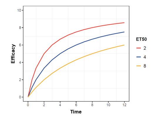
图 10.1 不同 ET50 对模型曲线的影响示意图#
10.2. 模型构建#
对于不含微分方程的模型(例如 Emax 模型),我们可以直接使用 Module 来构建模型:
class Soy(Module):
    def __init__(self, emax, et50, eta_emax, eta_et50, eps):
        self.pop_emax = theta(emax, bounds=(-200, -0.01))
        self.pop_et50 = theta(et50, bounds=(0.01, 12))

        self.eta_emax = omega(eta_emax)
        self.eta_et50 = omega(eta_et50)

        self.eps = sigma(eps)

        self.t = column("TIME")
        self.sample = column("SAMPLE")

    def pred(self):
        emax = self.pop_emax * exp(self.eta_emax)
        et50 = self.pop_et50 * exp(self.eta_et50)

        eff = (emax * self.t) / (et50 + self.t)
        ipred = eff

        w = 1 / self.sample**0.5  # 根据样本量对残差加权
        y = ipred + w * self.eps

        return y
model = PopModel(Soy(emax=-50, et50=3, eta_emax=0.5, eta_et50=0.5, eps=10), data=soy_isoflavone)
[MTran] Start interpreting module: Soy
[MTran] Interpretation finished in 0.802712 seconds
10.3. 模型拟合#
我们使用 FOCEi 算法来拟合模型:
fit_res = model.fit(FOCEi(print=10))
[MTran] Vaporization started for Soy(Module)
[MTran] Vaporization finished in 0.195993 seconds
➡️ Since build cache already exists, skip compile
✈️ First Order Conditional Estimation
Using BFGS...
* maxiter = 9999
* xtol = 1e-06
* ftol = 1e-06
* lower_bounds =
* upper_bounds =
* log_level = 0
* print = 10
* print_type = 0
* verbose = 1
* p_small = 0.1
* rel_step_size = 0.001

# 0    ofv: 237.3966213
Params:       1.0000e-01  1.0000e-01  1.0000e-01  1.0000e-01  1.0000e-01
NParams:     -5.0000e+01  3.0000e+00  7.0711e-01  7.0711e-01  3.1623e+00
Gradients:    8.8899e+01  1.7254e+01  3.3415e+01  4.8810e+00  1.1754e+01
Funcalls:   5
# 1    ofv: 237.331643
Params:       6.4538e-02  9.3117e-02  8.6670e-02  9.8053e-02  9.5311e-02
NParams:     -5.1341e+01  2.9846e+00  6.9774e-01  7.0573e-01  3.1475e+00
Gradients:    8.4708e+01  1.6569e+01  3.1414e+01  4.7312e+00  1.0045e+01
Funcalls:   12
converged = True
n_iter = 9
x_opt =   2.4051e-01 -1.5410e-02 -2.1643e-01  4.0180e-02  6.9227e-02
f_opt = 229.9503657
fun_calls = 93
message: Minimization success

Estimation Summary

────────────────────────────────────────────────────────────────────────────────
    Step         OFV
────────────────────────────────────────────────────────────────────────────────
✅ Converged 229.950
────────────────────────────────────────────────────────────────────────────────


Parameter Estimation

────────────────────────────────────────────────────────────────────────────────
 Parameter     Estimate   Shrinkage(%)
────────────────────────────────────────────────────────────────────────────────
Theta
  pop_emax     -44.918
  pop_et50     2.749
Omega(SD)
  eta_emax     0.515        3.047
  eta_et50     0.666        26.008
Sigma(SD)
  eps          3.066        20.759
────────────────────────────────────────────────────────────────────────────────


Information

────────────────────────────────────────────────────────────────────────────────
 Number of       Time
 Iterations
────────────────────────────────────────────────────────────────────────────────
9            0:00:00.19
────────────────────────────────────────────────────────────────────────────────

Estimation finished, now start covariance calculation.
Computing Covariance...
Covariance computation succeed
fit_res
Estimation Summary
| Estimation | Covariance | OFV |
|---|---|---|
| ✅ Converged | ✅ Succeed | 229.950 |
| Number of Observations: | 156 | |
| Number of Parameters: | 5 | |
Parameter Estimation
| Parameter | Estimate | RSE(%) | Shrinkage(%) |
|---|---|---|---|
| Theta | |||
| pop_emax | -44.918 | 9.082 | |
| pop_et50 | 2.749 | 16.006 | |
| Omega(SD) | |||
| eta_emax | 0.515 | 9.702 | 3.047 |
| eta_et50 | 0.666 | 13.242 | 26.008 |
| Sigma(SD) | |||
| eps | 3.066 | 9.425 | 20.759 |
Information
| Number of Iterations | Time | ||
|---|---|---|---|
| Compilation | Estimation | Covariance | |
| 9 | 0:00:00.20 | 0:00:00.19 | 0:00:00.22 |
fit_res.plot_gof()
根据本次拟合的参数估计结果,我们来更新基础模型的参数初值并重新拟合,以获取更准确的参数估计值:
est = fit_res.estimates
est
| Parameter | Value |
|---|---|
| Theta | |
| pop_emax | -44.918 |
| pop_et50 | 2.749 |
| Omega(SD) | |
| eta_emax | 0.515 |
| eta_et50 | 0.666 |
| Sigma(SD) | |
| eps | 3.066 |
model = fit_res.fork()
fit_res = model.fit(FOCEi(print=10))
[MTran] Vaporization started for Soy(Module)
[MTran] Vaporization finished in 0.082031 seconds
➡️ Since build cache already exists, skip compile
✈️ First Order Conditional Estimation
Using BFGS...
* maxiter = 9999
* xtol = 1e-06
* ftol = 1e-06
* lower_bounds =
* upper_bounds =
* log_level = 0
* print = 10
* print_type = 0
* verbose = 1
* p_small = 0.1
* rel_step_size = 0.001

converged = True
n_iter = 3
x_opt =   9.9816e-02  9.9850e-02  1.0007e-01  1.0003e-01  9.9973e-02
f_opt = 229.9503617
fun_calls = 42
message: Minimization success

Estimation Summary

────────────────────────────────────────────────────────────────────────────────
    Step         OFV
────────────────────────────────────────────────────────────────────────────────
✅ Converged 229.950
────────────────────────────────────────────────────────────────────────────────


Parameter Estimation

────────────────────────────────────────────────────────────────────────────────
 Parameter     Estimate   Shrinkage(%)
────────────────────────────────────────────────────────────────────────────────
Theta
  pop_emax     -44.926
  pop_et50     2.749
Omega(SD)
  eta_emax     0.515        3.049
  eta_et50     0.666        26.005
Sigma(SD)
  eps          3.066        20.756
────────────────────────────────────────────────────────────────────────────────


Information

────────────────────────────────────────────────────────────────────────────────
 Number of       Time
 Iterations
────────────────────────────────────────────────────────────────────────────────
3            0:00:00.11
────────────────────────────────────────────────────────────────────────────────

Estimation finished, now start covariance calculation.
Computing Covariance...
Covariance computation succeed
fit_res
Estimation Summary
| Estimation | Covariance | OFV |
|---|---|---|
| ✅ Converged | ✅ Succeed | 229.950 |
| Number of Observations: | 156 | |
| Number of Parameters: | 5 | |
Parameter Estimation
| Parameter | Estimate | RSE(%) | Shrinkage(%) |
|---|---|---|---|
| Theta | |||
| pop_emax | -44.926 | 9.083 | |
| pop_et50 | 2.749 | 16.009 | |
| Omega(SD) | |||
| eta_emax | 0.515 | 9.704 | 3.049 |
| eta_et50 | 0.666 | 13.249 | 26.005 |
| Sigma(SD) | |||
| eps | 3.066 | 9.425 | 20.756 |
Information
| Number of Iterations | Time | ||
|---|---|---|---|
| Compilation | Estimation | Covariance | |
| 3 | 0:00:00.8 | 0:00:00.11 | 0:00:00.24 |
上述结果表明,模型参数估计结果已收敛且较为准确,可以进行下一步分析。
10.4. 协变量筛选与模型评价#
在 MBMA 研究中,由于被纳入分析的文献或临床试验中的受试者人口学特征及试验设计方法差异较大,往往会导致报道结果间的异质性(heterogeneity)。为了保证分析结果的可靠性,我们需要通过探索和构建协变量(covariates)模型来识别和测量这些异质性,以解释药效学参数的变异来源,明确药物行为的影响因素,增强结果的可靠性和临床意义。
考察的协变量应具有一定的临床意义或符合药物的药理机制,常考察的协变量包括:人口学特征(如年龄、体重、种族)、疾病状态(如基线值、疾病周期)、试验设计方案(如对照药类型、试验中心数、制剂类型)、治疗相关因素(如合并用药、辅助疗法)等。本例中将考察的协变量为:AGE、BASELINE、CENTRE、YEAR。此外,也需要决定将被引入协变量的固定效应参数——一般选择具有较强临床意义和可解释性的参数。在本例中我们将仅在 Emax 参数上引入协变量。
目前最常用的协变量筛选方法为 SCM 法(stepwise covariates modeling)。SCM 法中包括前向引入(forward selection)与逆向剔除(backward selection)的两个过程(图 10.2)。在向前引入过程中,将待筛选的协变量逐个引入至模型固定效应参数上,观察引入后模型目标函数值(objective function value,OFV)是否有显著下降;保留能最显著降低 OFV 的一个协变量于模型中,随后重复尝试逐个引入余下的协变量,直至 OFV 不再显著降低。逆向剔除过程中,则将逐个剔除已被引入模型的协变量,观测剔除后 OFV 是否有显著上升;剔除令 OFV 上升最少的一个协变量,随后重复逐个剔除剩余的协变量,直至 OFV 不再显著上升。在两个步骤中均能使 OFV 显著变化的协变量将会保留在模型中,此时的模型即为最终模型。
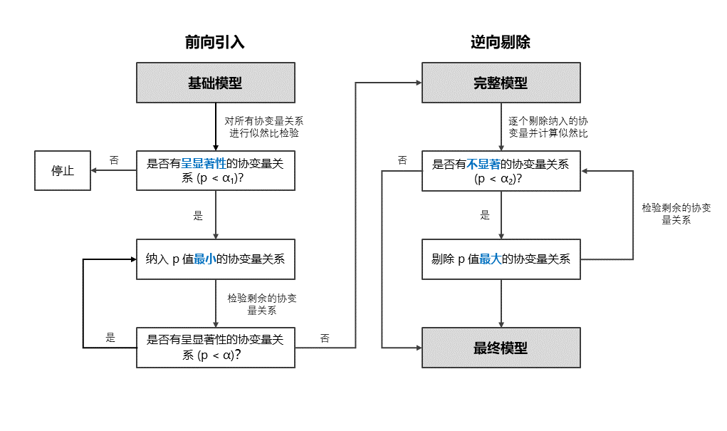
图 10.2 SCM 法步骤示意图#
参考文献
Jonsson, E. N., & Karlsson, M. O. (1998). Automated covariate model building within NONMEM. Pharmaceutical research, 15(9), 1463–1468.
在将协变量引入模型之前,我们需要先考虑协变量间的相关性。对于两两间存在较强相关性的协变量,应只考察其中一个,以避免共线性问题影响最终结果。使用 plot_covariates() 可以绘制协变量相关性矩阵图:
cov_mat = plot_covariates(soy_isoflavone, categorical_names=["CENTRE", "YEAR"], exclude_names=["SAMPLE"])
cov_mat.with_layout(width=720, height=600)
观测上述相关性计算结果可以发现,
YEAR与其他的变量相关性较强。在后续 SCM 法中将仅考察除了YEAR外的协变量。
若要进行 SCM 法,我们需要编写一个 SCM 法设置。与定义模型参数类似,我们在函数内定义需要考察的协变量及其类型(例如是否为分类变量),以及考察的协变量-参数关系与引入形式。例如:
@scm.spec
def rules(m: Soy):
    age = column("AGE")
    baseline = column("BASELINE")
    centre = column("CENTRE", is_categorical=True)

    # 设置连续变量的筛选策略
    scm.test_cont(covariates=[age, baseline], on=m.pop_emax, states=["exclude", "linear", "exp", "power"])

    # 设置分类变量的筛选策略
    scm.test_cat(covariates=centre, on=m.pop_emax, states="*")
编写配置时的部分要点如下:
使用
@scm.spec装饰器来说明此函数内包含需要被测试的协变量-参数关系。在
scm.test()中定义需要考察的协变量-参数关系与引入形式;若想考察所有可能的引入形式,可直接使用states="*"。
配置编写完成后,使用 scm() 方法即可执行 SCM 法:
scm_res = fit_res.scm(rules)
scm_res
运行完成后,可以使用
final_model查看最终模型:
final_model = scm_res.final_model
final_model
class Soy__4_3(Module):
    def __init__(self):
        super().__init__()

        # Define thetas
        self.pop_emax = theta(-46.42, bounds=(-200.0, -0.01))
        self.pop_et50 = theta(2.793, bounds=(0.01, 12.0))
        self.BASELINE__pop_emax_1 = theta(0.4137, bounds=(-0.5555555555555556, 0.8333333333333333))

        # Define etas
        self.eta_emax = omega(0.1716)
        self.eta_et50 = omega(0.4775)

        # Define epsilons
        self.eps = sigma(9.368)

        # Define covariates (data columns)
        self.t = column("TIME")
        self.sample = column("SAMPLE")
        self.AGE = column("AGE")
        self.BASELINE = column("BASELINE")
        self.CENTRE = column("CENTRE", is_categorical=True)
    def pred(self):
        AGE__pop_emax = 1
        # Linear BASELINE on pop_emax
        BASELINE__pop_emax = 1 + self.BASELINE__pop_emax_1 * (self.BASELINE - 4.5)
        CENTRE__pop_emax = 1
        # pop_emax with covariates
        pop_emax__with_cov = self.pop_emax * AGE__pop_emax * BASELINE__pop_emax * CENTRE__pop_emax
        emax = pop_emax__with_cov * exp(self.eta_emax)
        et50 = self.pop_et50 * exp(self.eta_et50)

        eff = (emax * self.t) / (et50 + self.t)
        ipred = eff

        w = 1 / self.sample**0.5  # 根据样本量对残差加权
        y = ipred + w * self.eps

        return y
SCM 完成后,我们仍需要检查最终模型的参数估计结果并对最终模型进行模型评价,以保证最终模型参数估算准确且模型较为稳定。
final_fit_res = scm_res.final_fit_result
final_fit_res
Estimation Summary
| Estimation | Covariance | OFV |
|---|---|---|
| ✅ Converged | ✅ Succeed | 215.684 |
| Number of Observations: | 156 | |
| Number of Parameters: | 6 | |
Parameter Estimation
| Parameter | Estimate | RSE(%) | Shrinkage(%) |
|---|---|---|---|
| Theta | |||
| pop_emax | -46.420 | 7.602 | |
| pop_et50 | 2.793 | 15.849 | |
| BASELINE__pop_emax_1 | 0.414 | 21.427 | |
| Omega(SD) | |||
| eta_emax | 0.414 | 11.800 | 6.127 |
| eta_et50 | 0.691 | 14.234 | 22.316 |
| Sigma(SD) | |||
| eps | 3.061 | 9.397 | 20.726 |
Information
| Number of Iterations | Time | ||
|---|---|---|---|
| Compilation | Estimation | Covariance | |
| 15 | 0:00:00.9 | 0:00:00.48 | 0:00:00.33 |
p_gof = final_fit_res.plot_gof()
p_gof
vpc_res = final_fit_res.vpc()
vpc_res.plot()
Running Auto-bin...
Bin search ended, result is 7
Auto-bin completed, finally use 5 bins.
bs_res = final_fit_res.bootstrap(500)
|=====|=====|=====|=====|=====|=====|=====|=====|=====|=====| 50
|=====|=====|=====|=====|=====|=====|=====|=====|=====|=====| 100
|=====|=====|=====|=====|=====|=====|=====|=====|=====|=====| 150
|=====|=====|=====|=====|=====|=====|=====|=====|=====|=====| 200
|=====|=====|=====|=====|=====|=====|=====|=====|=====|=====| 250
|=====|=====|=====|=====|=====|=====|=====|=====|=====|=====| 300
|=====|=====|=====|=====|=====|=====|=====|=====|=====|=====| 350
|=====|=====|=====|=====|=====|=====|=====|=====|=====|=====| 400
|=====|=====|=====|=====|=====|=====|=====|=====|=====|=====| 450
|=====|=====|=====|=====|=====|=====|=====|=====|=====|=====| 500
Bootstrap data sampling...
✅ Bootstrap complete.
bs_res
Bootstrap Summary
| Success Rate (%) | Elapsed Time |
|---|---|
| 100.000 | 0:03:43.22 |
Parameter Summary
| Parameter | Estimate | Median | 95%CI |
|---|---|---|---|
| Theta | |||
| pop_emax | -46.420 | -46.782 | -54.043, -39.769 |
| pop_et50 | 2.793 | 2.767 | 1.982, 3.908 |
| BASELINE__pop_emax_1 | 0.414 | 0.405 | 0.204, 0.551 |
| Omega(SD) | |||
| eta_emax | 0.414 | 0.402 | 0.300, 0.503 |
| eta_et50 | 0.691 | 0.656 | 0.453, 0.850 |
| Sigma(SD) | |||
| eps | 3.061 | 3.008 | 2.426, 3.537 |
上述结果表明,SCM 法得到的最终模型参数估算准确、拟合良好,且预测性能与稳定性均较优,可以作为最终模型并进行模型模拟。
这也提示我们,基线时患者的平均潮热发作频率将显著影响大豆异黄酮治疗潮热的最大效应——当患者基线发作频率越高时,大豆异黄酮越能降低潮热发作频率。
10.5. 模型模拟#
当最终模型构建完成后,可以使用它来模拟不同场景下的大豆异黄酮药效典型值。
例如欲了解患者基线发作频率分别为 3.5、4.0、4.5 次/天时大豆异黄酮在 12 周时可降低多少发作率,我们可以构建如下模拟场景:
import numpy as np

scenario = pl.DataFrame(
    {
        "ID": np.repeat([1, 2, 3], 13),
        "TIME": np.tile(np.arange(0, 13, 1), 3),
        "BASELINE": np.repeat([3.5, 4, 4.5], 13),
        "SAMPLE": np.repeat([100], 13 * 3),
        "GROUP": np.repeat(["Low", "Median", "High"], 13),
    }
)
scenario = scenario.cast({"GROUP": pl.Enum(["Low", "Median", "High"])})
scenario
| ID | TIME | BASELINE | SAMPLE | GROUP |
|---|---|---|---|---|
| i32 | i32 | f64 | i32 | enum |
| 1 | 0 | 3.5 | 100 | "Low" |
| 1 | 1 | 3.5 | 100 | "Low" |
| 1 | 2 | 3.5 | 100 | "Low" |
| 1 | 3 | 3.5 | 100 | "Low" |
| 1 | 4 | 3.5 | 100 | "Low" |
| … | … | … | … | … |
| 3 | 8 | 4.5 | 100 | "High" |
| 3 | 9 | 4.5 | 100 | "High" |
| 3 | 10 | 4.5 | 100 | "High" |
| 3 | 11 | 4.5 | 100 | "High" |
| 3 | 12 | 4.5 | 100 | "High" |
可以通过
final_model.fit_result.simulate()来使用最终模型参数估计结果进行模拟:
final_model
class Soy__4_3(Module):
    def __init__(self):
        super().__init__()

        # Define thetas
        self.pop_emax = theta(-46.42, bounds=(-200.0, -0.01))
        self.pop_et50 = theta(2.793, bounds=(0.01, 12.0))
        self.BASELINE__pop_emax_1 = theta(0.4137, bounds=(-0.5555555555555556, 0.8333333333333333))

        # Define etas
        self.eta_emax = omega(0.1716)
        self.eta_et50 = omega(0.4775)

        # Define epsilons
        self.eps = sigma(9.368)

        # Define covariates (data columns)
        self.t = column("TIME")
        self.sample = column("SAMPLE")
        self.AGE = column("AGE")
        self.BASELINE = column("BASELINE")
        self.CENTRE = column("CENTRE", is_categorical=True)
    def pred(self):
        AGE__pop_emax = 1
        # Linear BASELINE on pop_emax
        BASELINE__pop_emax = 1 + self.BASELINE__pop_emax_1 * (self.BASELINE - 4.5)
        CENTRE__pop_emax = 1
        # pop_emax with covariates
        pop_emax__with_cov = self.pop_emax * AGE__pop_emax * BASELINE__pop_emax * CENTRE__pop_emax
        emax = pop_emax__with_cov * exp(self.eta_emax)
        et50 = self.pop_et50 * exp(self.eta_et50)

        eff = (emax * self.t) / (et50 + self.t)
        ipred = eff

        w = 1 / self.sample**0.5  # 根据样本量对残差加权
        y = ipred + w * self.eps

        return y
sim_res = final_fit_res.simulate(data=scenario)
sim_res
[WARNING] 'AGE' not found in given data but is required in model. Filling with None values
[WARNING] Casting AGE to numeric dtype
[WARNING] 'CENTRE' not found in given data but is required in model. Filling with None values
[WARNING] Casting CENTRE to numeric dtype
Summary
| N Subject | N Obs | Seed | Simulation Time |
|---|---|---|---|
| 3 | 39 | 1234 | 0:00:00.0 |
我们使用图形来比较不同基线水平下大豆异黄酮群体药效典型值。从下图中可以发现:当患者基线发作频率为 3.5、4.0、4.5 次/天时,大豆异黄酮在 12 周时可分别降低 22.08%、29.87%、37.66% 的发作频率。根据此模拟结果,可在后续研究中进一步比较大豆异黄酮与其他药物的疗效差异。
p_sim_ind = (
    sim_res.plot_ind(y_name="_PRED_")
    .with_labels(x="Time (wk)", y="Typical Effect (%)", title="Simulated Typical Effect")
    .with_facet_wrap("GROUP")
)
p_sim_ind